The Types of Cell Elements
Each cell in a Gnumeric worksheet can contain only a single data element. These elements will have one of five basic types: text, numbers, booleans, formulas, or errors. During data entry, Gnumeric assigns a default data type to the cell based on an analysis of the cell contents. This assignment can be changed later if Gnumeric makes the wrong assignment. For information on how to change the data type of a cell, see Section 5.10 ― Formatting Cells.
The five basic types of data which can be stored in a spreadsheet cell are:
- Text
-
A text element can contain a series of letters, numbers or other contents. For example, the first cell in a worksheet might contain the characters —This worksheet describes the company's income — which Gnumeric would interpret to be text. In order to distinguish text elements from number or formula elements, the text element may start with a single quote. For instance, if a cell contained only the three digits 345, Gnumeric would consider that to be the number three hundred and forty five. If this cell is intended to be a string, Gnumeric will store the cell as '345. The newline character cannot be entered directly but must be entered as Alt+Enter. For more information on entering and formatting text elements, see Section 5.2.1 ― Text Data Elements.
- Numbers
-
A number element can contain a series of digits (425) but may include specific text and formatting characters to indicate negative numbers (-345), decimal separator (34.0567), thousand separators (12,342), currency ($23), dates (21-10-1998), times (10:23) or scientific notation (2.3e12). Dates may include the names of months or their abbreviation. The currency, decimal separator and thousands separator symbols vary depending on the locale (the language and other location specific behaviour) to which Gnumeric has been set. See Section 13.5 ― Languages and Locales to understand how to change the locale. If you want a number to be displayed as a plain string without any number formatting, you can put a single quote (') before it. For more information on entering and formatting, numeric elements see Section 5.2.2 ― Number Data Elements.
- Boolean
-
A boolean element can contain one of two values: TRUE and FALSE. These are useful as inputs or outputs from formulas and for boolean algebra. More information on boolean data elements is presented in Section 5.2.3 ― Boolean Data Elements.
- Formulas
-
A formula is an instruction to Gnumeric which describes a calculation which should be performed automatically. These formulas can contain standard arithmetic elements but can also contain references to other cells. Calculations which depend on other cells are usually recalculated when the values of another cell changes. Formulas always begin with a special character — the equals sign (=). The commercial at symbol (@) can be used instead of the equals sign during data entry but Gnumeric will convert this to an equals sign. Alternatively, an entry which describes a calculation and which starts with either the plus (+) or minus symbol (-) will be converted to a formula starting with an equals sign. For a more complete explanation of formulas, see Section 5.2.4 ― Formula Elements.
A cell reference is the part of a formula which refers to another cell. For example, in the formula to add two cells =(A4+A1), both A4 and A1 are cell references. These references can be quite complex referring to cells in different worksheets or even in different files. See Section 5.2.4.3 ― Cell Referencing for a complete explanation of references.
- Error
-
An error element describes the failure to calculate the result of a formula. These values are rarely entered directly by a user but usually are the display given when a formula cannot be correctly calculated. See Section 5.2.5 ― Error Elements for a complete list of error values and their explanation.
A cell may display a series of hash marks (######). This indicates that the result is too wide to display in the cell given the current font setting and the current column width. When this occurs, the value in the cell can be seen in two ways. If the cell is selected, the value will appear in the data entry area (to the right of the equals button directly above the cell grid). Alternatively, the column containing the cell can be widened until the data contents become visible: select the whole column (by clicking on the column header) and choose .
- 5.2.1. Text Data Elements
- 5.2.2. Number Data Elements
- 5.2.3. Boolean Data Elements
- 5.2.4. Formula Elements
- 5.2.5. Error Elements
5.2.1. Text Data Elements
Text elements consist of an arbitrary sequence of characters or numbers entered into a cell. Because Gnumeric automatically recognizes certain sequences as numbers or formulas, certain sequences of characters (such as sequences containing only digits or a text element which starts with an equals sign) must be treated specially to have them considered text. In order to force any sequence to be considered text, the sequence can be started with an apostrophe symbol ('). Alternatively, the 'number' format of the cell can be specified to be 'text' before entering the characters, as explained in Section 5.10.1 ― Number Formatting Tab. Text elements are the simplest elements to enter into spreadsheet cells.
An example of a spreadsheet cell grid with cells containing text is given in Figure 5-1.
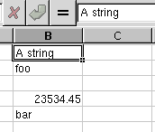
Valid text entries include simple words, whole sentences and even paragraphs.
To include a newline in a cell, a special key combination is required. A newline symbol can be inserted with the key combination of Alt+Enter.
5.2.2. Number Data Elements
Number data elements include a variety of data all of which are stored and manipulated by Gnumeric as numbers. This includes integers, decimal fractions, general fractions, numbers in scientific notation, dates, times, and currency values.
Data are recognized as numbers when they are entered, dependent on the format of the sequence of characters entered. Gnumeric attempts to intelligently guess the subtype of the data and match the data to an existing format for numbered data. If it matches a data format, Gnumeric will automatically assign the datum to a data type and associate an appropriate display format with the cell. The format recognition of Gnumeric includes a wide variety of data formats which are discussed in detail in Section 5.10.1 ― Number Formatting Tab.
Because Gnumeric automatically guesses the data type of a number being entered into a cell, this process may have to be over-ridden for certain types of data. For example, postal codes in the United States consist of a sequence of numbers which Gnumeric interprets as an integer. However, U.S. postal codes can start with a leading zero which Gnumeric discards by default. In order to override the default format, the number format of the cell must be specified before the entry of the data. This is explained in Section 5.10.1 ― Number Formatting Tab, below.
5.2.3. Boolean Data Elements
Cells can contain boolean data elements. These elements arise from Boolean logic which is a branch of mathematics. These elements are useful for manipulation of formulas.
Boolean values can be either "TRUE" or "FALSE". If these strings are entered into a cell, Gnumeric will recognize these as boolean values. These values can then be used in formulas. Certain formulas will also return boolean values.
5.2.4. Formula Elements
Formulas are the key to making a powerful spreadsheet. A formula instructs Gnumeric to perform calculations and display the results. These calculations are defined as a formula data elements. The power of these formulas arises because these formulas can include the contents of other cells and the results of the formulas are updated automatically when the contents of any cell included in the formula change. The contents of other cells are included using "cell references" which are explained below.
Any formula entered into a cell must follow a specific syntax so that Gnumeric can interpret the formula correctly. This syntax closely follows mathematical notation but also includes spreadsheet formulas, object names and cell references.
- 5.2.4.1. Syntax
- 5.2.4.2. Using Functions
- 5.2.4.3. Cell Referencing
- 5.2.4.4. Names
- 5.2.4.5. Array Formulas
- 5.2.4.6. Database Formulas
5.2.4.1. Syntax
Formulas are distinguished from regular data by starting with an equals sign (=) as the first character. Everything following this equals sign is evaluated as a formula.
To accommodate those more familiar with Lotus spreadsheets, Gnumeric recognizes the commercial at symbol (@) as the beginning of a formula and substitutes an equals sign. The plus and minus characters (+ and -) may also start formulas that involve calculation, but when used in front of a single number only indicate the sign of the number.
The simplest formulas just use the standard math operator and symbols. Addition, subtraction, multiplication, and division are represented by +, -, *, and /, just as you would expect. +,- can be placed in front of numbers to indicate sign, as well.
=5+5            returns 10.

=5-4            returns 1.

=-5             returns -5.

=5*5            returns 25.

=(5*5)+11       returns 36.

=(5*5)+(49/7)   returns 32.
Formulas can result in error values in several instances. If a formula is entered incorrectly, Gnumeric will display a warning and allow either the formula to be corrected or will save the formula as text for editing later. If a syntactically correct formula results in a nonsensical calculation (for instance, a division by zero), then an error value will be displayed indicating the error.
5.2.4.2. Using Functions
Formulas can also contain functions which denote the use of standard mathematical, business, statistical, and scientific calculations. These functions take the place of any data element in a formula and can therefore be combined with the standard arithmetic operators described above.
These functions have the form:
where FUNCTIONNAME indicates the name of a function and ARGUMENTS indicates one or more arguments to the function. The function arguments are separated by commas (,).While the documentation generally refers to functions and to cells in capital letters, their use is not actually case sensitive.
Some examples of the use of functions are:
The arguments of the functions vary in number from none, as in the PI() function, to an unlimited number, as in the SUM() function, depending on the type of function.5.2.4.3. Cell Referencing
Formulas can include the displayed data from other cells. These contents are described as `cell references' which are names indicating that the contents of other cells should be used in the calculation.
Each cell in a spreadsheet is named by its column and row labels. By default, the column labels are letters and the row labels are numbers. The first cell, therefore, is called A1. One column over and two rows down from cell A1 is the cell B3. In a worksheet of the default size, the right most and bottom most cell is cell IV65536 which is the cell in column IV and in row 65536. An alternative cell reference notation uses numbers for both row and column identification. See Section 5.2.4.3.2 ― References using R1C1 Notation below for details.
The value of a cell can be used in a formula simply by entering its name where a number value would otherwise occur. For example, to have the data in cell B1 appear in another cell, enter =B1 into that cell. Other more complex examples include:
- 5.2.4.3.1. Absolute cell referencing
- 5.2.4.3.2. References using R1C1 Notation
- 5.2.4.3.3. Referencing multiple cells
- 5.2.4.3.4. Referencing cells on other sheets
- 5.2.4.3.5. Referencing cells on other files
5.2.4.3.1. Absolute cell referencing
Cells can be referenced in the default way (relative referencing), or by using absolute referencing. Absolute referencing means that when the cell is copied, the cell reference does not change. Normally, auto-filling a cell range or moving a cell will change its cell reference so that it maintains a relation to the original cell. Absolute referencing prevents these changes.
The difference between absolute and relative cell references only matters if you are copying or moving cells that contain cell references. For cells that are going to remain in place, both the relative and absolute references have the same result.
For example, if =A1 is the formula entered into cell B2, cell B2 will display the data in cell A1, which is one row up and one column left. Then, if you copy the contents of B2 to cell F6, cell F6 will contain the value from E5, which is also one row up and one column left.
For the copied cell to still refer to A1, specify absolute references using the $ character: $A$1 refers to cell A1, no matter where it is copied.
The format for absolute cell referencing is to use a '$' in front of the cell coordinate that you want to stay constant. The column, the row, or both can be held constant.
What happens when a given formula is entered into cell B2, then copied to other cells?
- =A1
-
=A1 is a normal, or relative, cell reference function. When =A1 is entered into cell B2, it refers to the value of data one cell up and one cell left from the cell with the reference. Therefore, if this formula were copied from cell B2 to cell C2, the value displayed in cell C2 will be the value of data in cell B1. Copied to cell R19, the formula will display the data in cell Q18.
- =$A1
-
In this case, the column value is absolute, but the row value is relative. Therefore, if =$A1 is entered into cell B2, the formula refers to the data in column A that is one row up from the current location. Copied to cell C2, the formula will refer to the data in cell A1. Copied to cell R19, it will refer to the data in A18.
- =A$1
-
This formula uses a relative column value and an absolute row value. In cell B2, it refers to cell A1 as the data in the cell one column left and in row 1. Copied to cell C3, the formula will display the data in cell B1.
- =$A$1
-
No matter where this formula is copied, it will always refer to the data in cell A1.
5.2.4.3.2. References using R1C1 Notation
From the submenu you can select R1C1 notation for a worksheet. This causes all cell references on the sheet to be shown as “RrCc”, where r is the row number and c is the column number. When R1C1 notation is selected, the column headers show numbers rather than letters.
When r and c are positive integers, as in “R1C1”, the reference is absolute. To produce a relative reference, enclose a number in square brackets; if the number is zero, it can be omitted along with the brackets. For example, “RC[-2]” refers to the cell two columns to the left in the current row, while “R[1]C1” refers to the cell in the first column of the next row down from the referencing cell. The second example combines a relative row reference with an absolute column reference.
5.2.4.3.3. Referencing multiple cells
Many functions can take multiple cells as arguments. This can either be a comma separated list, an array, or any combination thereof.
- 5.2.4.3.3.1. Multiple individual cells
- 5.2.4.3.3.2. Referencing a continuous region of cells
- 5.2.4.3.3.3. Referencing non-continuous regions
5.2.4.3.3.1. Multiple individual cells
A comma separated list of cell references can be used to indicate cells that are discontinuous.

5.2.4.3.3.2. Referencing a continuous region of cells
For functions that take more than one argument, it is often easier to reference the cells as a group. This can include cells in sets horizontally, vertically, or in arrays.
The ':' operator is used to indicate a range of cells. The basic syntax is upper left corner:bottom right corner.

5.2.4.3.4. Referencing cells on other sheets
It is possible to reference cells which are not part of the current sheet. This is done using the SHEETNAME!CELLLIST syntax, where SHEETNAME is an identifier (usually a sheet name) and CELLLIST is a reference to a cell or range of cells as described in the previous sections. If SHEETNAME contains spaces or other special characters, you must quote the whole name to allow Gnumeric to recognize it as a single name. See the examples below.
When the reference is to a range of cells, the worksheet name only needs to be given with the first cell reference. The ending cell of the range is assumed to be on the same worksheet if an explicit sheet name is not specified. Note, however, that “Sheet1!A1:Sheet3!C5” is a legitimate cell range description. It identifies a range three columns wide and five rows deep on each of the worksheets from Sheet1 through Sheet3. The preferred form of such a reference is “Sheet1:Sheet3!A1:C5”, which is the form Gnumeric will display if you subsequently edit the contents of a cell containing such a reference.
5.2.4.3.5. Referencing cells on other files
It is possible to reference cells in other files. The canonical form for these references is [filename]SHEETNAME!CELLLIST. The square brackets serve to quote filename, so you should use quotation marks only if they are actually part of the file name. Note that the sheet name must be present in references of this form.
5.2.4.4. Names
Names are labels which have a meaning defined in the spreadsheet or by Gnumeric. A name can refer to a numeric value, a string, a range of cells, or a formula. For details on defining and using names, see Section 5.17 ― Defining Names.
5.2.4.5. Array Formulas
It is periodically useful or necessary to have an expression return a matrix rather than a single value. The first example most people think of are matrix operations such as multiplication, transpose, and inverse. A less obvious usage is for data retrieval routines (databases, realtime data-feeds) or functions with vector results (yield curve calculations).
5.2.4.6. Database Formulas
Solely for compatibility with Excel and ODF files, Gnumeric supports various database functions: DAVERAGE , DCOUNT , DCOUNTA , DGET , DMAX , DMIN , DPRODUCT , DSTDEV , DSTDEVP , DSUM , DVAR and DVARP .
Since these functions are quite restrictive on the criteria that can be used, it is often easier to use array functions as described in Section 5.2.4.5 ― Array Formulas. Array functions are also useful in the case that a specific database function does not exist:
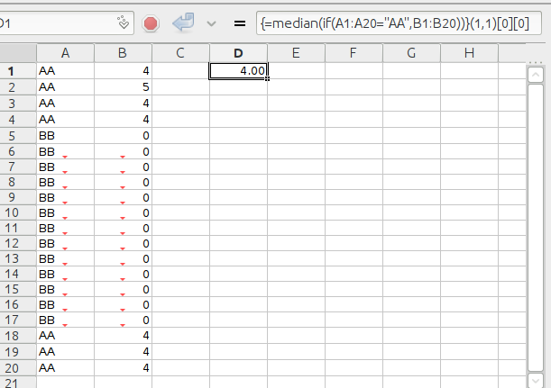
As shown in Figure 5-2, instead of using (the non-existing) function DMEDIAN one can use the alternative expression median(if(A1:A20="AA",B1:B20)) entered as an array function as described in Section 5.2.4.5 ― Array Formulas. Multiple conditions can be combined using multiplication to obtain AND and addition to obtain OR as in median(if((A1:A20="AA")+(C1:C20="BB"),B1:B20)). Using defined names as introduced in Section 5.2.4.4 ― Names for A1:A20 and B1:B20 can make this code very flexible and readable.
In this case we cannot use if(OR(A1:A20="AA",C1:C20="BB"),...) since the OR function would be applied to all 40 equality tests rather than each of the 20 pairs of equality tests.
5.2.5. Error Elements
Cells can display error values if the formula contained in the cell cannot be solved or if other anomalous conditions occur.
In Gnumeric all error values have names that start with #. 8 error values are standardized:
| Name | Normal Use |
|---|---|
| #DIV/0! | Division by zero occurred. |
| #N/A | Not applicable. This is the result of the =NA() formula. |
| #NAME? | An unknown function name or other name was encountered. |
| #NULL! | The result of specifying an intersecting range that in fact does not intersect. |
| #NUM! | A formula could not be evaluated because an invalid number was used as argument, for example =SQRT(-1) |
| #REF! | An invalid cell address or reference was encountered. |
| #UNKNOWN! | Usually the result of importing an unrecognized error from a different file format. |
| #VALUE! | A formula could not be evaluated because the wrong type of argument was used. |