Formatting Cells
This section describes how to format the appearance of data in a cell. The section Section 5.11 ― Conditional Formatting of Cells describes a more advanced method of formatting where the depends on various conditions involving the current cell value and/or the values in other cells.
Cell formats allow you to only change the way cell data appears in the spreadsheet. It is important to keep in mind that it only alters the way the data is presented, and does not change the value of the data.
The formatting options allows for monetary units, scientific options, dates, times, fractions,and more. Positive and negative values can have different colors and formats for aiding in keeping track of values. There are also a large variety of date and time formats for virtually any time and date format one can think of. Formatting also allows you to set font, background color, and borders for selected cells.
Finally, advanced formatting options allow you to lock some of the cells so that their values cannot be changed, or restrict the range of values that can be entered in the selected cells.
To change the formatting of a cell or a selection, you can either use the Format Cells dialog which holds all of the formatting options or use specific formatting elements available as buttons on the Format Toolbar.
This dialog, shown in Figure 5-16, gives you access to all formatting options.
To launch this dialog, select the cell or range of cells you want to format (see Section 5.6 ― Selecting Cells and Cell Ranges for details on selecting cells) and then use one of the following methods:
- Use keyboard shortcut Ctrl+1 (this is number one, not letter l).
- Choose in the menubar.
- Click with the right mouse button on the cell grid area and choose from the context menu.
The Format Cells dialog contains tabs Number, Alignment, Font, Border, Background, Protection, and Validation. These tabs are described in detail in the subsequent sections.
To set one of formatting options, select the corresponding tab, choose the options you need, and click . This will apply the options you selected (in all tabs) and close Format Cells dialog. You can also click on to apply the and keep the dialog open, or on to close the dialog without applying changes.
Some of the most commonly used formatting options, such as font, background, and alignment, can also be accessed by using the buttons in the Format Toolbar. This toolbar is described in detail in Section 4.4.3 ― The Format Toolbar,
- 5.10.1. Number Formatting Tab
- 5.10.2. Alignment, Font, Border, and Background Tabs
- 5.10.3. Protection and Validation Tabs
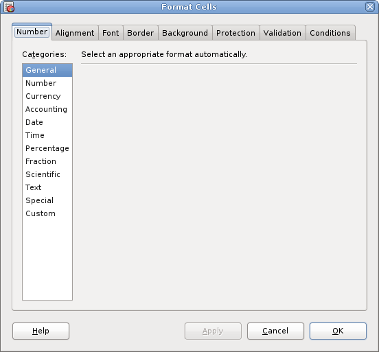
5.10.1. Number Formatting Tab
This tab allows you to select the format for the cell's contents. You can select one of the many preset formatting styles which should be more than adequate for the vast majority of cases. If none of these meet the needs of the user, it is possible to create your own formats.
To use one of the preset formats, select the format category (such as Number or Date) by clicking on the corresponding radiobutton in the left side of the dialog. The right side of the dialog will show you how the selected cell would look with this format and give more options for the selected format.
The following is a list of all available format categories:
- General
A Swiss army knife of a format. It will attempt to display a value it the 'best' way possible. The choice of format depends on the size of the cell and Gnumeric guess of what 'type' of value is being displayed (number, date, time ...).
- Number
Displays numbers with 0-30 digits after the decimal place. Negatives can be displayed normally, within parentheses, or in red color. Optionally a delimiter can be added every third order of magnitude (thousand, million, ...). Both the decimal point and the thousands separator have internationalization support.
- Currency
Similar to Number, with the addition of a currency symbol. Currently known symbols include $, ¥, £, ¤ and the three letter abbreviations of all major currencies. By default, Gnumeric will use currency symbol and placement (before or after the number) appropriate for your locale.
- Accounting
A specialization of Currency which pays more attention to the alignment of negative numbers. It ensures that a small amount of space is prepended to positive numbers so that they align with negatives.
- Date
This category contains various formats for presenting dates. By default, Gnumeric will use date format appropriate for your locale (country and language setting). You can also choose one of many possible date formats shown in the list in the right side of the dialog. The following is an explanation of codes used in these formats:
Some date formats also include time using the codes explained below. Examples of date formatting are shown in Table 5-2.- d: day of month (one or two digits). Example: 9.
- dd: day of month (two digits). Example: 09.
- ddd: day of week. Example: Wed.
- m: month (number, one or two digits). Example: 3.
- mm: month (number, two digits). Example: 03.
- mmm: month (abbreviated name). Example: Mar.
- mmmm: month (full name). Example: March.
- mmmmm: month (first letter). Example: M.
- yyyy: year (four digits). Example: 1967.
- yy: last two digits of year. Example: 67.
- Time
This category contains various formats for presenting time of day. You can choose one of many possible time formats shown in the list in the right side of the dialog. The following is an explanation of codes used in these formats:
Sometimes it is necessary to display more than 24 hours, or more that 60 minutes/seconds without the values incrementing the display unit of the next larger measure (e.g., 25 hours instead of 1 day + 1 hour). To achieve this, use codes '[h]', '[mm]', and '[ss]'. Examples of time formatting are shown in Table 5-3.- h: hours.
- mm: minutes.
- ss: seconds.
- Percentage
Multiplies a value by 100 and appends a percent. Can be used with 0-30 digits after the decimal place.
- Fractions
Approximate the value with a rational number with either a specific denominator or with a maximum number of digits in the denominator.
- Scientific
Formats the value using scientific notation, e.g. 5.334 E 6 for 5,334,000. Allows up to 30 digits after the decimal place. No provision for controlling the exponent are provided at this time.
- Text
-
Treats numeric values as text. This will show a number with as much precision as available and will lose knowledge of whether it represented a date, or time.
TIPIf your workbook contains serial numbers, ID numbers or other similar entries, choose Text format for them. If you choose General or Number format, Gnumeric will remove leading zeros, so that 01124 will be shown as 1124.
- Custom
This category allows you to define your own format. This is only recommended for advanced users as it requires understanding of the codes internally used by Gnumeric for describing formats. To make it easier, this category provides a list of codes for all predefined formats so you can create our own format by modifying one of them rather than starting from scratch.
| Format | Sample | ||
|---|---|---|---|
| General | 36068.755 | ||
| m/d/yy | d/m/yy | 9/30/98 | 30/9/98 |
| m/d/yyyy | d/m/yyyy | 9/30/1998 | 30/9/1998 |
| d-mmm-yy | mmm-d-yy | 30-Sep-98 | Sep-30-98 |
| d-mmm-yyyy | mmm-d-yyyy | 30-Sep-1998 | Sep-30-1998 |
| d-mmm | mmm-d | 30-Sep | Sep-30 |
| d-mm | mm-d | 30-09 | 09-30 |
| mmm/d | d/mmm | Sep/30 | 30/Sep |
| mm/d | d/mm | 09/30 | 30/09 |
| mm/dd/yy | dd/mm/yy | 09/30/98 | 30/09/98 |
| mm/dd/yyyy | dd/mm/yyyy | 09/30/1998 | 30/09/1998 |
| mmm/dd/yy | dd/mmm/yy | Sep/30/98 | 30/Sep/98 |
| mmm/dd/yyyy | dd/mmm/yyyy | Sep/30/1998 | 30/Sep/1998 |
| mmm/ddd/yy | ddd/mmm/yy | Sep/Wed/98 | Wed/Sep/98 |
| mmm/ddd/yyyy | ddd/mmm/yyyy | Sep/Wed/1998 | Wed/Sep/1998 |
| mm/ddd/yy | ddd/mm/yy | 09/Wed/98 | Wed/09/98 |
| mm/ddd/yyyy | ddd/mm/yyyy | 09/Wed/1998 | Wed/09/1998 |
| mmm-yy | Sep-98 | ||
| mmm-yyyy | Sep-1998 | ||
| mmmm-yy | September-98 | ||
| mmmm-yyyy | September-1998 | ||
| d/m/yy h:mm | m/d/yy h:mm | 9/30/98 18:07 | 30/9/98 187:07 |
| d/m/yyyy h:mm | m/d/yyyy h:mm | 9/30/1998 18:07 | 30/9/1998 187:07 |
| yyyy/mm/d | 1998/09/30 | ||
| yyyy/mmm/d | 1998/Sep/30 | ||
| yyyy/mm/dd | 1998/09/30 | ||
| yyyy/mmm/dd | 1998/Sep/30 | ||
| yyyy-mm-d | 1998-09-30 | ||
| yyyy-mmm-d | 1998-Sep-3 | ||
| yyyy-mm-dd | 1998-09-30 | ||
| yyyy-mmm-d | 1998-Sep-30 | ||
| yy | 98 | ||
| yyyy | 1998 | ||
5.10.2. Alignment, Font, Border, and Background Tabs
- 5.10.2.1. Alignment Tab
- 5.10.2.2. Font Tab
- 5.10.2.3. Border Tab
- 5.10.2.4. Background Tab
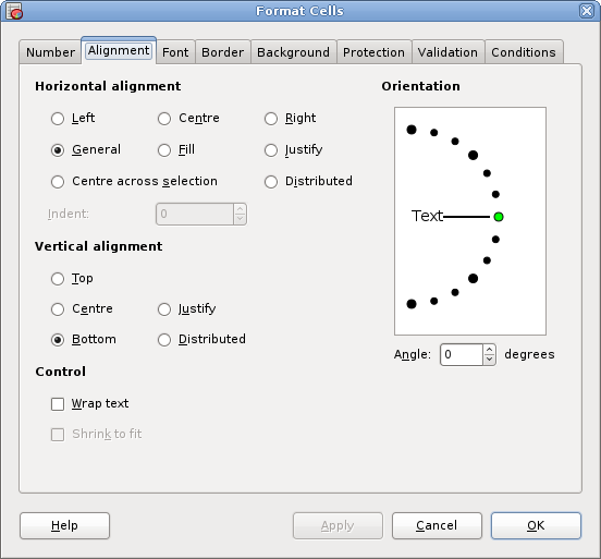
5.10.2.1. Alignment Tab
This tab allows you to set horizontal and vertical alignment and justification options.
-
The standard default justification. Use right justification for numbers and formulas, and left justification for text strings.
-
Left justify all cell contents.
-
Center all cell contents.
-
Right justify all cell contents.
-
Fill the cell with the contents. This will repeat the cell's contents as necessary to fill the width of the cell.
-
For text, wrap long lines of text and left justify. For other formats, same as Left.
-
Centers the cell's contents so the middle of each line is aligned with the middle of other lines. This only works with multiple cells.
Left and Right justification options also allow you to specify indent from left (respectively, right) side of the cell. Indent is measured in multiples of the current font size: for font size 10, indent 4 means 40 pts.
-
Align the top of the cells contents with the top of the cell.
-
Center the cells contents vertically. Equally space between the top and bottom.
-
Align the contents of the cell with the bottom of the cell.
-
For text, wrap long lines and spread lines of text evenly to fill the cell. For other formats (or if the text contains no long lines), same as Bottom justification.
5.10.2.2. Font Tab
This tab allows you to change the font used for cells content.
To change cells font, select font family (such as Times, Helvetica, etc), style (Normal, Bold, ...) and size in points. You can also select font color and special effects such as underlining or strikethrough.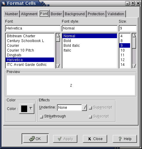
Gnumeric allows you to use any of the fonts known to GNOME printing system, gnome-print. The same fonts are used for screen display and for printing, assuring that the printed document will look identical to the one you see on screen. Advanced users can refer to documentation for gnome-print package to find out more about adding fonts and font management in GNOME.
A quicker way to change the selected cells' font is to use Format Toolbar.
5.10.2.3. Border Tab
This tab allows you to choose the border for the selected cells. You can select one of many border styles (none, single line, double line,...) and colors. You can also have different borders on different sides of the cell.
To choose a border for a cell or a selection, select border style and color in the right side of the tab and click on the buttons corresponding to the sides of the cells in the left side of the tab. In addition to the buttons for left, right, top, and bottom sides, you also have buttons for drawing diagonal and reverse diagonal of the cell. (Strictly speaking, these cannot be called borders, but it is natural to put them in this tab.) The lowest row of buttons contains buttons and . Clicking on removes all borders from the cell; clicking on puts border on all sides of the cell or selection.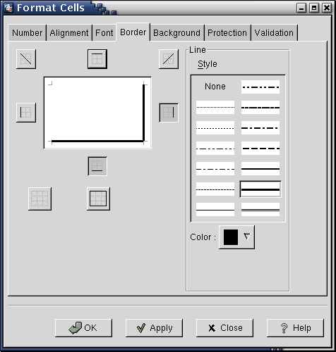
Please note that for a selection of cells, the buttons will put borders on one of the sides of selection, not of individual cells. For example, clicking on button will put the border along the bottom of the selection, so only the cells in the bottom row will be affected. In addition for selections you have three more buttons in the bottom row: , , and . puts borders on all inside vertical borders in the selection; puts borders on all inside horizontal borders in the selection, and puts borders on all inside borders in the selection, both vertical and horizontal.
To remove an existing border from one of the sides of a cell or selection, click on the corresponding button again.
5.10.2.4. Background Tab
This tab allows you to change the background of selected cells. You can choose solid color or patterned background. A preview of the selected background will be shown in the right part of the tab.
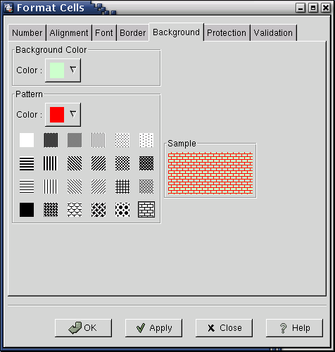
To select a solid color background, select the color from Background Color drop-down box. You can use of the standard colors or define your own color by clicking on button.
To select a patterned background, choose the background color in Background Color section. After this, choose the pattern color and type in Pattern section. Please note that the pattern type buttons use black pattern on white background, regardless of the colors you have chosen.
To remove pattern, choose Solid pattern type (top left button, looking like a white square).
5.10.3. Protection and Validation Tabs
These two tabs are used to control user's access to cells and restrict values of data allowed in a cell. Unlike other formatting options, these two tabs have no effect on a cells appearance. These options are mostly used for writing templates and forms to be filled by others.
- 5.10.3.1. Protection Tab
- 5.10.3.2. Validation Tab
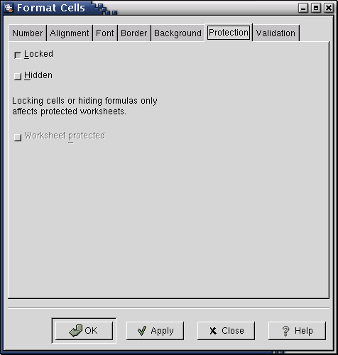
5.10.3.1. Protection Tab
This tab allows you to see and change cell protection in imported Excel workbooks. Cell protection has no effect in Gnumeric: you can edit cells whether or not they are marked as protected. However, Gnumeric keeps the protection setting of imported Excel workbooks. If you later save your workbook in Excel format, Gnumeric will save the protection information too. For more information about cell protection in Excel, please refer to Excel documentation.
5.10.3.2. Validation Tab
This tab allows you to set restrictions on allowed values of data in the cells. If you (or someone else) attempts to enter a data that does not meet the set criteria, a warning (or an error message, depending on the options set in this tab) will be shown.
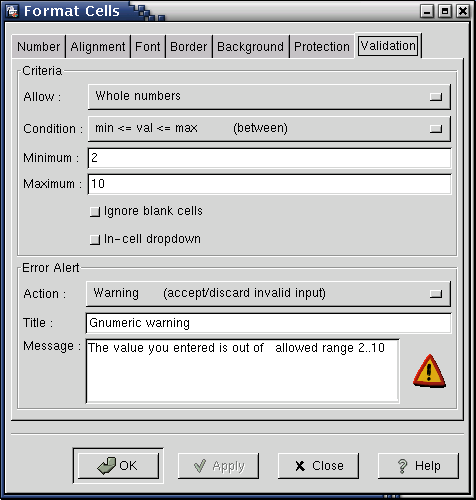
This tab consists of two part. The first part, Criteria is used to set the criteria for the cell values. The second part, Error Alert, is used to choose the action when data entered does not meet the criteria.
To set the criteria for cell values, follow these steps:
-
Choose the type of data contained in the cells, using the Allow drop-down list.
-
Choose a condition that must be satisfied by the cells value, using Condition drop-down list. In these conditions, val stands for the cells value (for text, val stands for the length of text string) and min, max, and bound are constants that you need to specify.
-
Enter the values of constants used in condition. For example, if you chose condition min<=val<=max , you need to enter values of constants min and max.
After specifying the criteria, you need to specify how Gnumeric should respond to incorrect cell value. You can choose one of four possible actions from Action drop-down list:
- None
Accept invalid value without any warning. Equivalent to having no validation.
- Stop
Do not accept the invalid value. Show the user an error message which you need to specify (see below).
- Warning
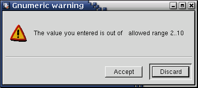
Show the user a warning dialog, giving him a choice whether to accept or reject the invalid value. You need to specify the message to use in the warning dialog (see below).
- Information
Accept invalid values but show the user a warning dialog. You need to specify the message to use in the warning dialog (see below).
If you choose one of the options Stop, Warning, or Information, you must enter the message that will be show to the user in the error or warning dialog. Otherwise, the dialog will be empty so it will be completely useless. You need to enter the title (which will be used as the window title for the dialog window) and the message itself. For example, the values shown in Section 5.10.3.2 ― Validation Tab will produce the dialog shown in Figure 5-23.