Dependent Observations
- 8.4.1. Forecast Tools
- 8.4.2. Fourier Analysis Tool
- 8.4.3. Kaplan Meier Estimates Tool
- 8.4.4. Principal Component Analysis
- 8.4.5. Regression Tool
8.4.1. Forecast Tools
- 8.4.1.1. Exponential Smoothing Tool
- 8.4.1.2. Moving Average Tool
8.4.1.1. Exponential Smoothing Tool
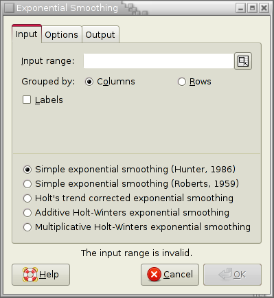
The Exponential Smoothing tool performs the exponential smoothing for the given set or sets of values. It provides the choice of 5 different exponential smoothing methods:
- Simple exponential smoothing according to (Hunter, 1968).
- Simple exponential smoothing according to (Roberts, 1959).
- Holt's trend corrected exponential smoothing (occasionally also referred to as double exponential smoothing)
- Additive Holt-Winters exponential smoothing
- Multiplicative Holt-Winters exponential smoothing (occasionally also referred to as triple exponential smoothing)
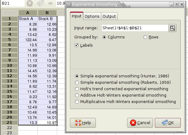
Since the kind of options available depend on the type of exponential smoothing desired, you can choose the type on the “Input ” page.
- 8.4.1.1.1. Common Options of the Exponential Smoothing Tool
- 8.4.1.1.2. Exponential Smoothing According to Hunter
- 8.4.1.1.3. Exponential Smoothing According to Roberts
- 8.4.1.1.4. Holt's Trend Corrected Exponential Smoothing
- 8.4.1.1.5. Additive Holt-Winters Method
- 8.4.1.1.6. Multiplicative Holt-Winters Method
8.4.1.1.1. Common Options of the Exponential Smoothing Tool
Specify the cells containing the datasets in the “Input Range” entry. The entered range or ranges are grouped into datasets either by rows or by columns.
If you have labels in the first cell of each data set, select the “Labels” option.
If you select the “Include chart” option, Gnumeric will also create a chart showing both the data and corresponding smoothed values.
8.4.1.1.2. Exponential Smoothing According to Hunter
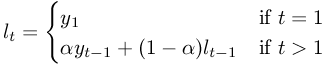
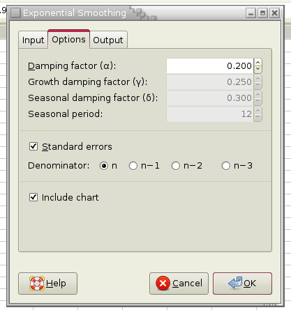
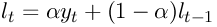
Each value in the smoothed set is predicted based on the forecast for the prior period. The formula is given in Figure 8-35. α is the value given as “Damping factor”. yt is the tth value in the original data set and lt the corresponding smoothed value.
For example, a value for α between 0.2 and 0.3 represents 20 to 30 percent error adjustment in the prior forecast.
If you choose to have the tool enter formulæ rather than values into the output region, then you can modify the damping factor α even after you executed the tool.
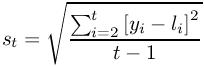
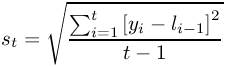
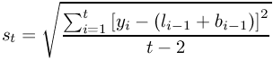
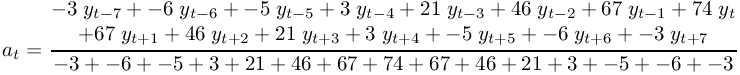
To have the standard errors output as well, check the “Standard error” check box. The formula used is given in Figure 8-36. The denominator can be adjusted by selecting the appropriate radio button. Since there are t−1 terms in the sum of the denominator, selecting “n−1” means that the denominator will be t−2.
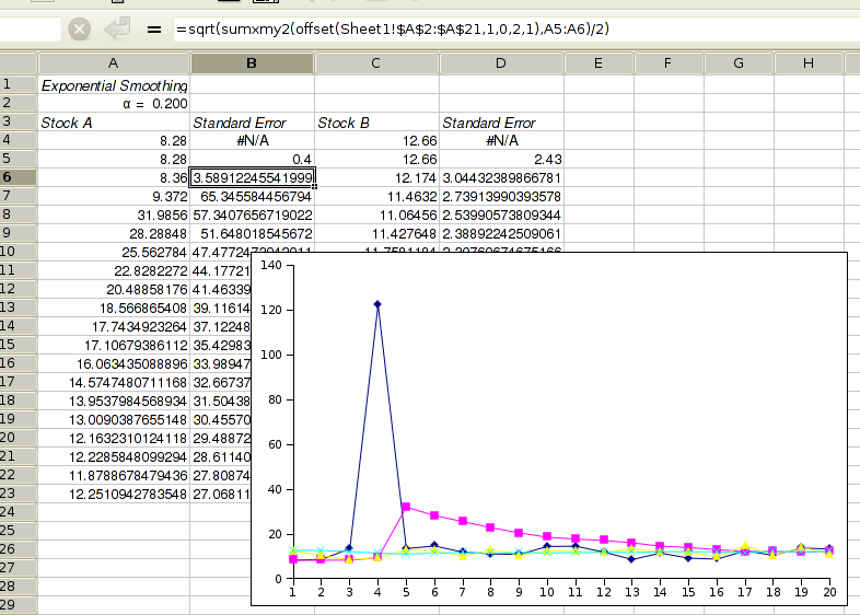
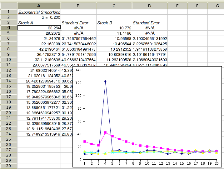
If you check the “Include chart” check box, a line graph showing the observations yt and the predicted values lt will also be created.
Figure 8-37 shows some example data, Figure 8-38 the selected options and Figure 8-39 the corresponding output.
8.4.1.1.3. Exponential Smoothing According to Roberts
The simple exponential smoothing method according to Roberts is used for forecasting a time series without a trend or seasonal pattern, but for which the level is nevertheless slowly changing over time. The predicted values are calculated according to the formula given in Figure 8-40. α is the value given as “Damping factor”. yt is the tth value in the original data set and lt the predicted value. l0 is the predicted value at time 0 and must be estimated. This tool uses the average value of the first 5 observations as estimate.
If you choose to have the tool enter formulæ rather than values into the output region, then you can modify the damping factor α and the estimated value at time 0 after executing the tool.
To have the standard errors output as well, check the “Standard error” check box. The formula used is given in Figure 8-41. The denominator can be adjusted by selecting the appropriate radio button.
If you check the “Include chart” check box, a line graph showing the observations yt and the predicted values lt will also be created.
Figure 8-42 shows example output for the exponential smoothing tool using the formula according to Roberts. Cell A4 contains the estimated level at time 0. If you requested to have formulæ rather than values entered into the sheet, then changing the estimate in A4 and/or the value for α in A2 will result in an immediate change to the predicted values.
8.4.1.1.4. Holt's Trend Corrected Exponential Smoothing
Holt's trend corrected exponential smoothing is appropriate when both the level and the growth rate of a time series are changing. (If the time series has a fixed growth rate and therefore exhibits a linear trend, a linear regression model is more appropriate.)
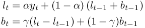
yt is the true value at time t, lt is the estimated level at time t and bt is the estimated growth rate at time t. We use the two smoothing equations given in Figure 8-43 to update our estimates. α is the value given as “Damping factor” and γ is the value given as “Growth damping factor”.
This tool obtains initial (time 0) estimates for the level and growth rate by performing a linear regression using the first 5 data values.
If you choose to have the tool enter formulæ rather than values into the output region, then you can modify the damping factors α and γ as well as the estimated level and growth rate at time 0 after executing the tool.
To have the standard errors output as well, check the “Standard error” check box. The formula used is given in Figure 8-44. The denominator can be adjusted by selecting the appropriate radio button.
If you check the “Include chart” check box, a line graph showing the observations yt and the estimated level values lt will also be created.
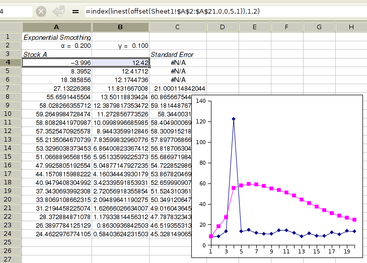
Figure 8-45 shows example output for Holt's trend corrected exponential smoothing. Cell A4 contains the estimated level at time 0 and B4 the estimated growth rate at time 0. If you requested to have formulæ rather than values entered into the sheet, then changing the estimates in A4, B4, the values for α in A2 and/or for γ in B2 will result in an immediate change to the predicted values.
8.4.1.1.5. Additive Holt-Winters Method
The additive Holt-Winters method of exponential smoothing is appropriate when a time series with a linear trend has an additive seasonal pattern for which the level, the growth rate and the seasonal pattern may be changing. An additive seasonal pattern is a pattern in which the seasonal variation can be explained by the addition of a seasonal constant (although we allow for this constant to change slowly.)
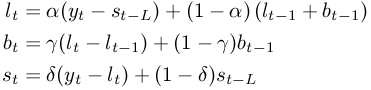
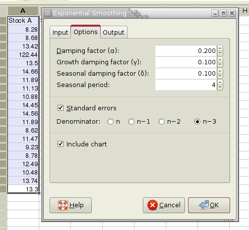
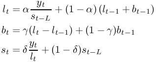
yt is the true value at time t, lt is the estimated level at time t, bt is the estimated growth rate at time t and st is the estimated seasonal adjustment for time t. We use the three smoothing equations given in Figure 8-46 to update our estimates. α is the value given as “Damping factor”, γ is the value given as “Growth damping factor” and δ is the value given as “Seasonal damping factor”. L is the value given as “Seasonal period”. If your data consist of monthly values, then L should be 12, if it consist of quarterly values then L should be 4.
This tool obtains initial (time 0) estimates for the level and growth rate by performing a linear regression using all data values. It obtains estimates for the seasonal adjustments by averaging the appropriate seasonal differences from values predicted by linear regression alone.
If you choose to have the tool enter formulæ rather than values into the output region, then you can modify the damping factors α, γ and δ as well as all estimates after executing the tool.
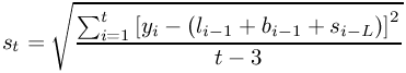
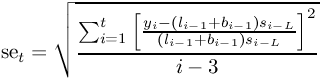
To have the standard errors output as well, check the “Standard error” check box. The formula used is given in Figure 8-47. The denominator can be adjusted by selecting the appropriate radio button.
If you check the “Include chart” check box, a line graph showing the observations yt and the estimated level values lt will also be created.
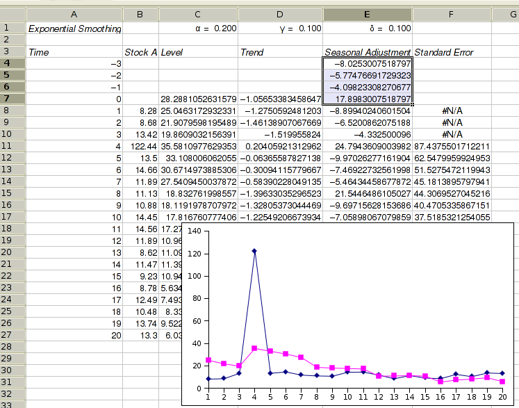
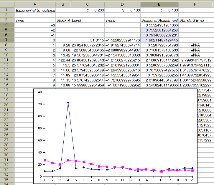
Figure 8-48 shows the options' tab of the exponential smoothing tool for the additive Holt-Winters method. The data is expected to have a seasonal period of 4 (this would for example happen if we have a data value for each quarter of a year). Figure 8-49 shows the corresponding example output for the additive Holt-Winters method. Cell C7 contains the estimated level at time 0, D7 the estimated growth rate at time 0, and E4 to E7 the initial seasonal adjustments for each of the 4 seasons preceding our data time period. If you requested to have formulæ rather than values entered into the sheet, then changing any of these estimates, the values for α in A2, for γ in B2 and/or for δ in C2 will result in an immediate change to the estimated values.
8.4.1.1.6. Multiplicative Holt-Winters Method
The multiplicative Holt-Winters method of exponential smoothing is appropriate when a time series with a linear trend has a multiplicative seasonal pattern for which the level, the growth rate and the seasonal pattern may be changing. A multiplicative seasonal pattern is a pattern in which the seasonal variation can be explained by the multiplication of a seasonal constant (although we allow for this constant to change slowly.)
yt is the true value at time t, lt is the estimated level at time t, bt is the estimated growth rate at time t and st is the estimated seasonal adjustment for time t. We use the three smoothing equations given in Figure 8-50 to update our estimates. α is the value given as “Damping factor”, γ is the value given as “Growth damping factor” and δ is the value given as “Seasonal damping factor”. L is the value given as “Seasonal period”. If your data consist of monthly values, then L should be 12, if it consist of quarterly values then L should be 4.
This tool obtains initial (time 0) estimates for the level and growth rate by performing a linear regression using the data values of the first 4 seasonal periods. It obtains estimates for the seasonal adjustments by averaging the appropriate seasonal differences from values predicted by linear regression alone during the first 4 seasonal periods.
If you choose to have the tool enter formulæ rather than values into the output region, then you can modify the damping factors α, γ and δ as well as all estimates after executing the tool.
To have the standard errors output as well, check the “Standard error” check box. The formula used is given in Figure 8-51. The denominator can be adjusted by selecting the appropriate radio button.
If you check the “Include chart” check box, a line graph showing the observations yt and the estimated level values lt will also be created.
Figure 8-52 shows the example output for the multiplicative Holt-Winters method, assuming 4 seasons. Cell C7 contains the estimated level at time 0, D7 the estimated growth rate at time 0, and E4 to E7 the initial seasonal adjustments for each of the 4 seasons preceding our data time period. If you requested to have formulæ rather than values entered into the sheet, then changing any of these estimates, the values for α in A2, for γ in B2 and/or for δ in C2 will result in an immediate change to the estimated values.
8.4.1.2. Moving Average Tool
Use the moving average tool to calculate moving averages of one or more data sets. A moving average provides useful trend information of the data that is lost in a simple average. In addition, moving averages can be used to eliminate random variance. For example, use this tool to create a smoother curve of a stock prize.
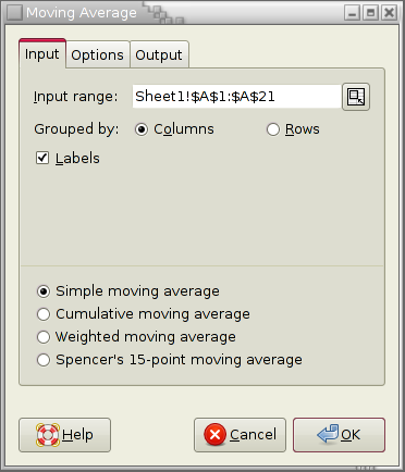
Specify the cells containing the datasets in the “Input Range” entry. The entered range or ranges are grouped into datasets either by rows or by columns.
If you have labels in the first cell of each data set, select the “Labels” option.
Choose the type of moving average you would like to calculate. The tool can determine 4 types of moving averages:
- Simple moving average
- Cumulative moving average
- Weighted moving average
- Spencer's 15 point moving average
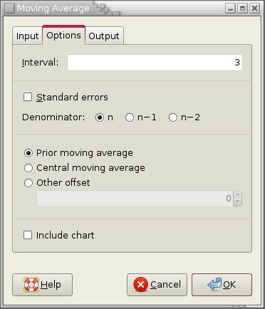
Specify the “Interval” for the moving average. The interval i is the number of consecutive values to be included in each moving average. This options is only available for the simple and weighted moving averages.
Check the “Standard errors” checkbox if you would also like the standard error to be calculated. Since there is no general agreement on the denominator for the standard error you can choose the appropriate radio button.
In the case of the simple moving average, you can also choose between a prior moving average and a central moving average, or you may even specify any other desired offset.
- “Prior moving average”: Each average takes into account the current observation and the most recent prior observations for a total of i observations.
- “Central moving average” with i being odd: Each average takes into account the current observation and the same number of most recent prior observations and closest future observations for a total of i observations.
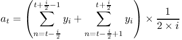
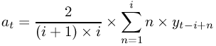
- “Central moving average” with i being even: This is calculated according to the formula given in Figure 8-55. at is the moving average at time t and yt is the observation at time t.
- “Other offset”: If the offset is 0, this is just the prior moving average. Otherwise the offset indicates the number of closest future observations to include in the average. Correspondingly, the number of most recent past observations is decreased.
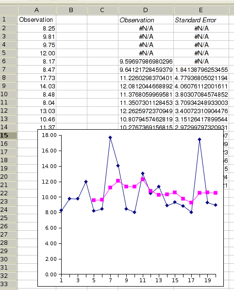
The results are given in one column for each dataset (with a second column added if you have chosen standard errors to be calculated). Each row represents the moving average of the corresponding row or column in the input range. Depending on the type of average and the offset, the moving average cannot be calculated for the first rows in the input range.
- 8.4.1.2.1. Simple Moving Average
- 8.4.1.2.2. Cumulative Moving Average
- 8.4.1.2.3. Weighted Moving Average
- 8.4.1.2.4. Spencer's 15 Point Moving Average
- 8.4.1.2.5. A Moving Average Example
8.4.1.2.1. Simple Moving Average
A simple moving average is the unweighted average of a collection of observations. Exactly which observations are included depends on whether a prior or central moving average is calculated.
8.4.1.2.2. Cumulative Moving Average
A cumulative moving average is a prior moving average in which the current and all prior observations are included.
8.4.1.2.3. Weighted Moving Average
A weighted moving average with an interval i is a prior moving average calculated according to formula Figure 8-55. at is the moving average at time t and yt is the observation at time t.
8.4.1.2.4. Spencer's 15 Point Moving Average
Spencer's 15 point moving average is a central moving average calculated according to formula Figure 8-57. at is the moving average at time t and yt is the observation at time t.
8.4.1.2.5. A Moving Average Example
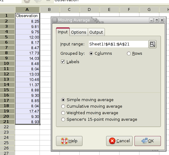
Figure 8-58 shows some example data, Figure 8-59 shows the option settings, and Figure 8-60 the corresponding output.

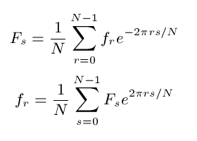
8.4.2. Fourier Analysis Tool
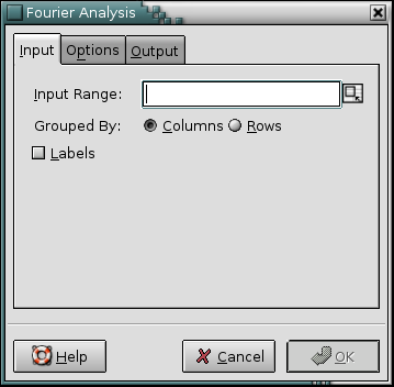
The Fourier Analysis tool normally performs a Fast Fourier Transform to obtain the discrete fourier transform Fs of the given sequence ft of real numbers according to the formula given in Figure 8-62.
Select the “Inverse” option to calculate the inverse discrete fourier transform ft of the given sequence Fs of real numbers
If the number of terms in the given sequence is not a power of 2 (i.e. 2, 4, 8, 16, 32, 64, 128, etc.), this tool will append zeros to reach such a power of 2!
Specify the cells containing the datasets in the “Input Range” entry. The entered range or ranges are grouped into sequences either by rows or by columns.
If you have labels in the first cell of each data set, select the “Labels” option.
Before using the numbers obtained by this tool, ensure that these are in fact the correct formulae for your discipline. In the physical sciences this fourier transform tends to be called the inverse fourier transform and vice versa. Moreover, frequently the scaling factor varies.
For example Mathematica uses the terms fourier transform and inverse fourier transform with the reversed meaning than Gnumeric and it uses a scaling factor of 1/SQRT(N) rather than 1/N.
8.4.3. Kaplan Meier Estimates Tool
- 8.4.3.1. The “Input” Tab
- 8.4.3.2. The “Groups” Tab
- 8.4.3.3. The “Options” Tab
- 8.4.3.4. The “Output” Tab
- 8.4.3.5. A Kaplan-Meier Example
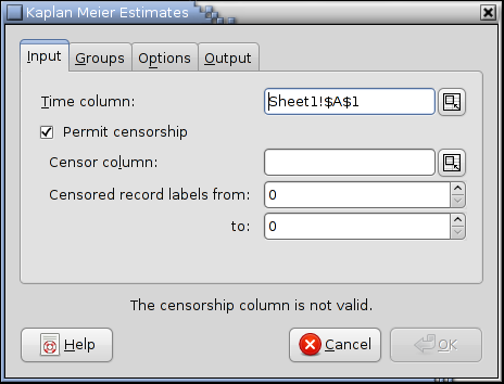
8.4.3.1. The “Input” Tab
The “Input” tab shown in Figure 8-63 contains the fields specifying the data to be used for the Kaplan Meier Estimates. The time column contains the times or dates at which the subjects died or were censored. If any of the subjects were censored, the Permit censorship checkbox is checked and the Censor column contained the censorship marks. Censorship marks are typically 0s or 1s. The range of censor marks or labels can be set using the remaining two spinboxes.
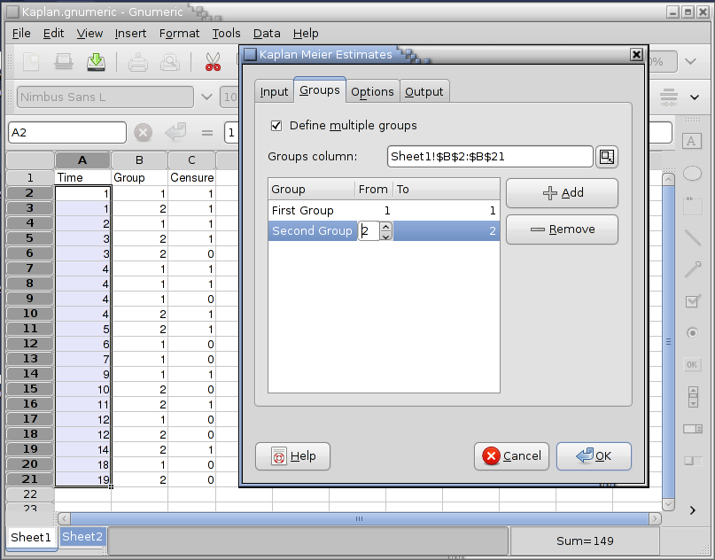
8.4.3.2. The “Groups” Tab
If the subjects belong to several groups and the groups are supposed to be analyzed separately, the groups tab can be used.
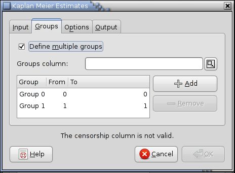
The groups tab can be enabled via the Define multiple groups checkbox. The groups column entry contains the address of the column specifying the group membership. Groups can then be defined or deleted via the Add and Remove buttons.
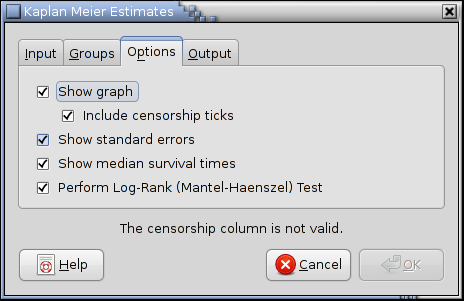
8.4.3.3. The “Options” Tab
The options tab of the Kaplan-Meier tools dialog is used to set various options of the Kaplan-Meier tool.
8.4.3.4. The “Output” Tab
The Output tab contains the standard output options and fields described in Section 8.1 ― Overview.
8.4.3.5. A Kaplan-Meier Example
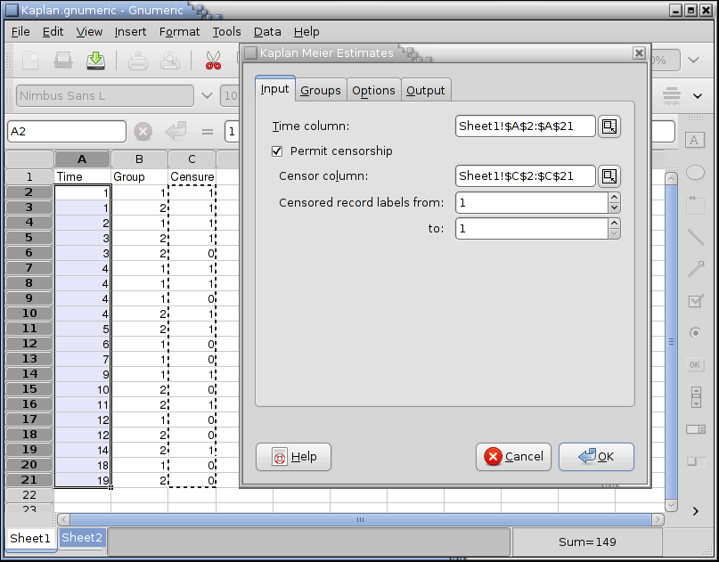
Suppose you want to calculate Kaplan-Meier Estimates for the as given in Figure 8-66. Each row contains the data for one subject. Column A contains the survival time, i.e. the time until death or censure. Column B contains the group number, we are considering two groups of subjects. Column C indicates whether the subject died (0) or was censured (1).
We complete the fields of the Input tab as shown in Figure 8-66. The time column is A2:A21 and the censure column is C2:C21.
Since we have two groups of subjects, on the Groups tab we check the Define multiple groups check box and set up two groups with identifiers 1 and 2 in column B2:B21:
On the Options tab all checkboxes are pre-checked and we leave them that way to obtain a maximum amount of information.
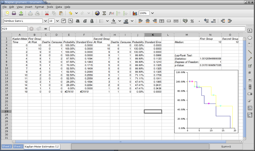
On the output tab we choose where we would like the output to be placed. For the purposes of this example we retain the New Sheet target. After clicking OK we get the output shown in Figure 8-68. Note that the graph initially always appears on top of the numerical result and was moved for the screen shot.
B1:F17 shows the results of the first group, G1 to K17 the results of the second group. The graph shows the Kaplan-Meier survival curves for both groups.
M4:N7 shows the result of the Mantel-Haenszel Log-Rank Test. In this case the p-value is larger than 0.3 and we would fail to reject the Null hypothesis. There is no evidence that the survival times differ.
8.4.4. Principal Component Analysis
Principal Component Analysis Tool performs a principal component analysis (PCA). PCA is a useful statistical technique with application in fields such as face recognition and image compression. It is a common technique for finding patterns in data of high dimension.
Specify the cells containing the datasets in the “Input Range” entry. The entered range or ranges are grouped into the factors either by rows or by columns.
If you have labels in the first cell of each factor, select the “Labels” option.
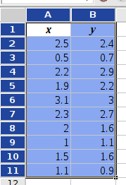
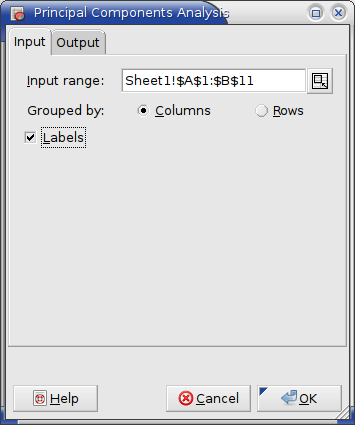
Suppose you want to perform a principal component analysis on the data given in Figure 8-70 having the two dimensions (factors) x and y.
- Enter Sheet1!$A$1:$B$11 (or just A1:B11) in the “Input Range:” entry by typing this directly into the entry or clicking in the entry field and then selecting the range on the sheet.
- Select the “” option since the first row contains labels. (see Figure 8-69).
- Specify the output options as described above.
- Press the OK button.
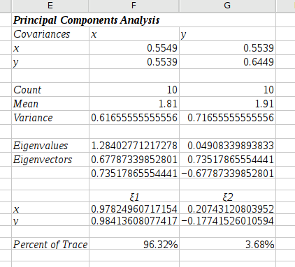
The output of this principal component analysis is shown in Figure 8-75. The output shows the covariance matrix, the eigenvalues and corresponding eigenvectors. The principal component is the constructed factor with the highest percent of trace, ξ1.
8.4.5. Regression Tool
The regression tool performs a multiple regression analysis.
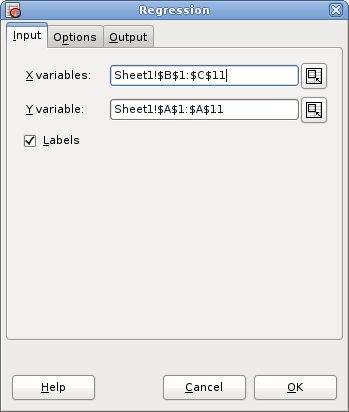
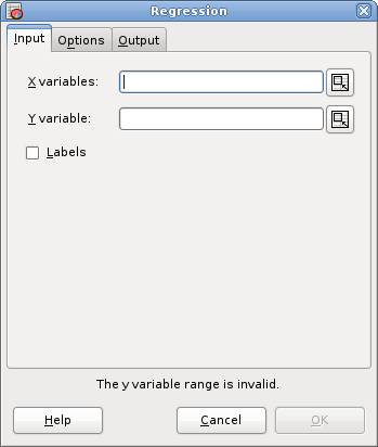
Enter a range or list of ranges containing the independent variables into the “X Variables:” entry.
Enter a single range containing the dependent variable into the “Y Variable:” entry.
If the ranges for the independent and dependent variables also contains labels in the first field of each row, column or area, select the “ Labels” option.
Specify the confidence level in the “Confidence Level:” entry. The default is 95%.
To force the regression line or plane to pass through the origin, select the “Force Intercept To Be Zero” option.
Specify the output options as described above. If the output is directed into a specific output range, that range should contain at least seven columns and 17 rows more than there are independent variables.
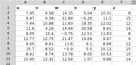
Suppose you want to perform a regression analysis on the data given in Figure 8-73 using v and y as independent variables and u as dependent variable.
- Enter B1:C11 in the “X Variables:” entry by typing this directly into the entry or clicking in the entry field and then selecting the range on the sheet.
- Enter A1:A11 in the “Y Variable:” entry.
- Select the “” option since the first row contains labels. (see Figure 8-74).
- Specify the output options as described above.
- Press the OK button.
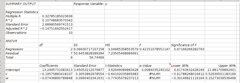
The output of this regression analysis is shown in Figure 8-75.