Solver
With Gnumeric Solver you can solve linear programs.
- 7.1.1. Introduction to Linear Programming
- 7.1.2. Spreadsheet Modeling
- 7.1.3. Using Solver
- 7.1.4. Integer Programming
7.1.1. Introduction to Linear Programming
A linear program (LP) is a problem that can be expressed as linear functions. As you probably already know, a linear function is the one whose graph is always a straight line. Thus each variable of it appears in a separate term with its coefficient. There must be no products or quotients of these variables. In addition, the exponent of each term must be one. No logarithmic, exponential, trigonometric terms are allowed. Especially note that functions like ABS, IF, MAX, and MIN are not linear. Here are a few examples of linear functions:
    3x + y - 5z
    -3.23x + 0.33y
    -0.3x + 4y - 2z + 1.2m
The linear problem has a so called objective function which is to be minimized or maximized and constraints. The objective function is the one whose value we would like to optimize. Typically, this function could determine the profit generated by the expected sales of the given model (maximization problem), or, the cost of the production in the given environment (minimization problem). Anyway, on purely mathematical point of view, we could examine the following objective function:
Maximize 2x + 3y - z
In linear programming the variables of this functions are not allowed to take any values (otherwise the maximum of any objective function would be infinity). The problem also has constraints. The constraints are a set of linear functions and a set of their right hand side values (RHS). For example, for the previously defined objective function we have the following constraints:
    x + y <= 5           (#1)
    3x - y + z <= 9      (#2)
    x + y >= 1           (#3)
    x + y + z = 4        (#4)
    x, y, z >= 0         (non-negativity assumption)
This constraint set consists of three inequality constraints (#1-#3) and one equality constraint (#4). Their RHS values are 5, 9, 1, and 4. In addition, we also have the non-negativity assumption. That is, all the variables (x, y, and z) have to take only positive numbers. The idea is to find the optimal values for the variables (x, y, and z) but also to satisfy all the given constraints.
7.1.2. Spreadsheet Modeling
To solve optimization problems with Gnumeric you have to type in the problem into a sheet. A recommended way to start with is to allocate a separate column in the spreadsheet for each decision variable (in the previous example the x, y, and z) and a separate row for each constraint (the constraints #1-#4). The coefficients of these variables should be placed into the cells corresponding to the allocated row and the column. It is also recommended that you label the rows and the columns to make the sheet much more readable. The sheet for our maximization problem would look like this:
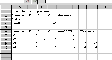
As you can see, we have put the model variables into cells B3:D3. They are currently all zeros. The cell E4 contains the objective function definition. The easiest way to define it is to use SUMPRODUCT build-in function. Thus in our model, we have the formula `=SUMPRODUCT(B3:D3,B4:D4)' in E3.
The constraints are defined in rows seven to ten. Since the coefficients of these functions are in columns B, C and D we will get the total sum of each of the constraint using the formula `SUMPRODUCT(B$3:D$3,Bn:Dn)' where n is the row number of the constraint. For example, in E7 we have `=SUMPRODUCT(B$3:D$3,B7:D7)', in E8 `=SUMPRODUCT(B$3:D$3,B8:D8)' and so on. The right hand side (RHS) values of the constraints are typed into cells G7:G10.
7.1.3. Using Solver
- 7.1.3.1. Solver Parameters
- 7.1.3.2. Solver Constraints
- 7.1.3.3. Solver Reporting
- 7.1.3.4. Optimization
7.1.3.1. Solver Parameters
Now it is time to select `Solver...' from the `Tools' menu. After you have done it, the following dialog will appear:
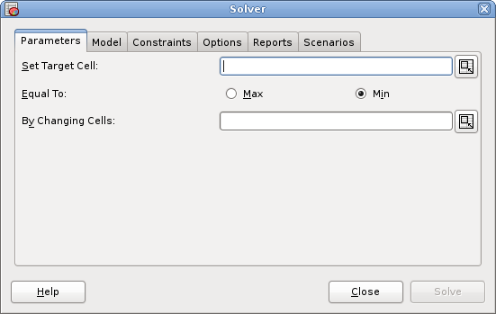
Since we have the objective function in E3 type this into the `Set Target Cell:' entry. We are about to maximize this function, thus the radio button `Max' should be pressed on. By default, the problem is assumed to be maximization problem. The input variables (x, y, and z) were in cells B3:D3 so type the cell range into the `By Changing Cells:' entry.
The model to be optimized is a linear model. Thus, we should check that the check button `Linear (LP/MILP)' is pressed on the page `Model'. Also make sure that the assume non-negative button is on, otherwise, the input variables can also take negative values. There is also a check button `Assume Integer (Discrete)' which adds an integer constraint for all the input variables. The integer optimization is described, however, later.
A few additional options can be set too. If you want to limit the number of iterations the optimization algorithm is allowed to take you can set the maximum number in the `Max iterations' entry box on page `Options'. Similarly, you can limit the maximum time the optimization is allowed to take in the `Max time' entry box. If either one of these settings is exceeded during the optimization, the optimization is interrupted and an error dialog is displayed.
Some models can be better solved if the model is scaled into another form before the actual optimization. Gnumeric solver supports automatic scaling which can be checked on by using the check button on the bottom of the dialog. Note that the automatic scaling does not change the model since before checking out the results the model is scaled back to its original form.
7.1.3.2. Solver Constraints
Now we can add the constraints. Select the `Constraints' page from the top of the dialog and the following page should appear.
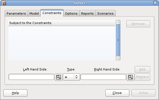
In this page, you can see all constraints that have been defined in the `Subject to the Constraints:' window. Since none has been defined, this window should be empty. Now type in the constraints (#1-#4) one by one.
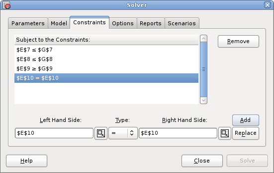
When adding constraints, the three entry boxes in the bottom of the dialog are used. Put a cell name of the total left hand side (LHS) cell into the `Left Hand Side:' entry box. In our example, this would be E7 for the constraint #1, E8 for constraint #2, and so on. The combo entry in the middle defines the type of the constraint. It can be `≤', `=', `≥' ,`Int' or `Bool'. We will explain the `Int' and `Bool' constraints later. In this example, you should select `≤' for constraints #1-#2, `≥' for #3, and `=' for constraint #4. The last entry on the right takes the right hand side values of the constraints. For constraints #1-#4 they should be G7 (5), G8 (9), G9 (1), and G10 (4) in this order.
After typing a constraint press button, and you will be able to define the next one. When you have typed in all the constraints, the Solver dialog should look like this:
The order of the constraints does not matter. If you want to change or delete a constraint click it and then press `Change' or `Delete' button.
Note that you can also type ranges into the LHS and RHS entries. For example, you could have typed D7:D8 and G7:G8 instead of the two separate constraints.
If the constraints have now been typed in correctly, we should check what reports we want to produce.
7.1.3.3. Solver Reporting
Select the `Reports' page from the top of the dialog and you will see a checkbox named `Program'. This report gives the model in its mathematical form. Program report is useful for checking out the correctness of the model. It can also be useful for educational purposes.
7.1.3.4. Optimization
After you have specified the parameters, the constraints and the reporting options it is time to press the button. If everything went ok, you will see a dialog saying: `Solver found an optimal solution. All constraints and optimality conditions are satisfied.'. This means that the solver found an optimal solution and the optimal values are now stored into the input variables. For all models, this, however, does not happen.
If a feasible solution cannot be found, the solver reports that `A feasible solution could not be found. All specified constraints cannot be met simultaneously.'.
If the model is unbounded, the solver reports that `The Target Cell value specified does not converge! The program is unbounded.'.
If the maximum number of iterations specified in the options was exceeded, the solver reports that `The maximum number of iterations exceeded. The optimal value could not be found.'.
If the maximum time specified in the options was exceeded, the solver reports that `The maximum time exceeded. The optimal value could not be found in given time.'.