Simulation Analysis
- 6.4.1. Introduction to simulation analysis
- 6.4.2. Setting up the simulation model
- 6.4.3. Running the simulation
- 6.4.4. Simulation output
- 6.4.5. Using SIMTABLE
- 6.4.6. Determining the number of iterations
6.4.1. Introduction to simulation analysis
A simulation is the imitation of the operation of a real-world process or system. The behavior of a system is studied by generating an artificial history of the system through the use of random numbers. These numbers are used in the context of a simulation model, which is the mathematical, logical and symbolic representation of the relationships between the objects of interest of the system. After the model has been validated, the effects of changes in the environment on the system, or the effects of changes in the system on system performance can be predicted using the simulation model. 1
Gnumeric includes a facility for performing Monte Carlo Simulation. Monte Carlo simulation involves the sampling of random numbers to solve a problem where the passage of time plays no substantive role. 2 In other words, each sample is not effected by prior samples. This is in contrast to discrete event simulation or continuous simulation where the results from earlier in the simulation can effect successive samples within a simulation experiment. The Monte Carlo simulation will be enabled through the use of the Random Number functions as described in ??? and the results presented along with statistics for use in analysis. 3
6.4.2. Setting up the simulation model
The remainder of this chapter will illustrate use of the simulation tool using an example from Banks et. al. 4 A classic inventory problem is the newsvendor problem. A newsvendor buys papers for 33 cents each and sells for 50 cents. Newspapers not sold are sold as scrap (recycled) for 5 cents. Newspapers are purchased by the paper seller in bundles of 10. Demand for newspapers can be categorized as “good,” “fair,” or “poor” with probability 0.35, 0.45 and 0.20 respectively, with each day's demand being independent of prior days. The problem for the newsvendor is to determine the optimal number of papers to purchase when the day's demand is not yet known.
The daily profit equation for the newsvendor is:
To set up the model, this example will use two tabs in Gnumeric, a tab labeled 'Profit' to calculate profit, and a tab labeled 'Demand Tables' to store the various tables needed to calculate the demand for any given sampling.
For the Profit tab, set up the profit tab as in Figure 6-1.
At the top of the Profit' tab, the Profit table will be entered . There are three variables: Sale revenue, Cost and Scrap value, and they take the per unit coefficients of 0.5, 0.33 and 0.05 respectively. Enter the coefficients in cells B13 through D13. In cells B12 through D12, enter the equations for sale revenue, cost and Scrap value that are in the list below. In cell E12, enter the equation for Profit
Next, we add the values for the decision variable, which is the amount purchased, and the amount sold.
- B12: =B13*min(B16,B20)
- C12: =C13*B16
- D12: =D13*max(0,B16-B20)
- E12: =B12-C12+D12
- B13: 0.5
- C13: 0.33
- D13: 0.05
- B16: 50

Sometimes, there is a need to try a number of different values for a single parameter. In Section 6.4.5 ― Using SIMTABLE the SIMTABLE function will be used to automate the use of a set of values for a parameter such as purchase quantity. For now, set the purchase quantity to 50 in cell C16.
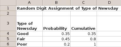
Next, create the demand tables from which the demand will be generated. In the tab 'Demand Tables' enter the values of the probability in cells B4 through B6 (B4: 0.35; B5: 0.45; B6: 0.2). In cells C4, C5 and C6 enter the cumulative probability values (C4: 0.35; C5: 0.8; C6: 1) as shown in Figure 6-2.
- B4: 0.35
- B5: 0.45
- B6: 0.2
- C4: 0.35
- C5: 0.8
- C6: 1.0
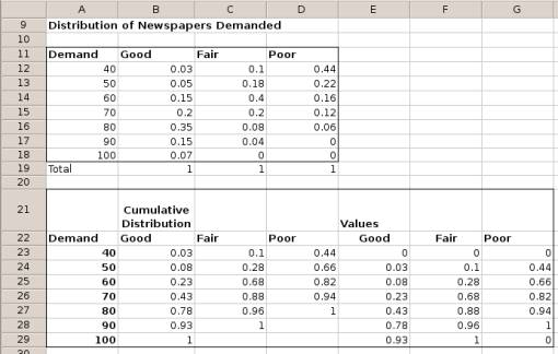
The next table is the daily demand for newspapers based on the type of news day. The table Distribution of Newspapers Demanded is in cells A11 through D18 of the Demand Tables worksheet as shown in Table 6-1 and contains the daily demand distribution values. The cumulative distribution tables in cells A21 through G29, shown in Table 6-2 are derived values from the Distribution of Newspapers Demanded using values in the top Distribution of Newspapers demanded table.
| A | B | C | D | |
| 11 | Demand | Good | Fair | Poor |
| 12 | 40 | 0.03 | 0.1 | 0.44 |
| 13 | 50 | 0.05 | 0.18 | 0.22 |
| 14 | 60 | 0.15 | 0.4 | 0.16 |
| 15 | 70 | 0.2 | 0.2 | 0.16 |
| 16 | 80 | 0.35 | 0.08 | 0.06 |
| 17 | 90 | 0.15 | 0.04 | 0 |
| 18 | 100 | 0.07 | 0 | 0 |
| A | B | C | D | E | F | G | |
| 21 | Cumulative Distribution | Values | |||||
| 22 | Demand | Good | Fair | Poor | Good | Fair | Poor |
| 23 | 40 | 0.03 | 0.1 | 0.44 | 0 | 0 | 0 |
| 24 | 50 | 0.08 | 0.28 | 0.66 | 0.03 | 0.1 | 0.44 |
| 25 | 60 | 0.23 | 0.68 | 0.82 | 0.08 | 0.28 | 0.66 |
| 26 | 70 | 0.43 | 0.88 | 0.94 | 0.23 | 0.68 | 0.82 |
| 27 | 80 | 0.78 | 0.96 | 1 | 0.43 | 0.88 | 0.94 |
| 28 | 90 | 0.93 | 1 | 0.78 | 0.96 | 1 | |
| 29 | 100 | 1 | 0.93 | 1 |
When these values are entered, the final results will look like Figure 6-3.
Finally, back in the Profit tab, the demand data will be filled in through the use of references to the Demand Tables tab as shown in Figure 6-4.
In the following cells, enter the equations below in the 'Profit' tab:
- B17: =rand()
- C17: =if(B17<'Demand Tables'!C4,"Good",if(C19<'Demand Tables'!C5,"Fair","Poor"))
- B18: =rand()
- B20: =lookup($C17,$B23:$D23,$B24:$D24)
- B21: =E12
- B24: =lookup(Profit!$B18,'Demand Tables'!E23:E29,'Demand Tables'!$A23:$A29)
- C24: =lookup(Profit!$B18,'Demand Tables'!F23:F29,'Demand Tables'!$A23:$A29)
- D24: =lookup(Profit!$B18,'Demand Tables'!G23:G29,'Demand Tables'!$A23:$A29)
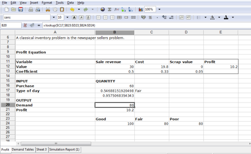
When done, the Profit spreadsheet will be setup with a profit equation, decision variables, and random events as shown in Figure 6-4. The rand() functions in cells C17 and C18 return a random value between 0 and 1, which are used by the lookup() functions in cells B20, B24, C24 and D24 to calculate a randomly determined daily demand. Next, this sheet will be used for analysis through the use of simulation.
6.4.3. Running the simulation
To run the simulation, from the Gnumeric toolbar, select Tools → Simulation. In the Risk Simulation dialog box that appears, the first tab is the Variables tab. There are two entries in the Variables tab: Input variables and Output variables (Figure 6-5).
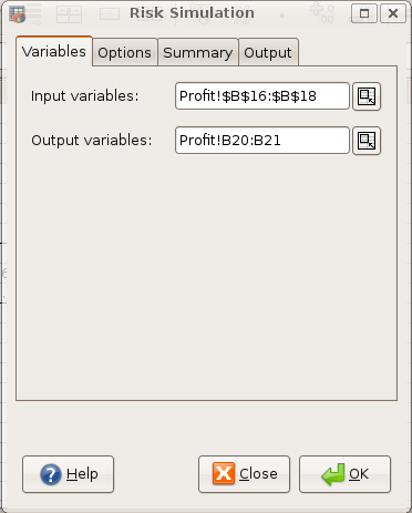
Input variables are the cells which hold the functions based on random numbers of the type described in Section A.14. In this case, they are the cells B17 and B18 in the Profit worksheet, which hold the rand() function. Later, when the quantity purchased is a parameter set by the SIMTABLE function, cell B16 which holds the purchase quantity will be added to the range of input variables.
Output variables are the results of interest, or the dependent variable. In this case, the dependent variables are the demand and the profit, which are in cells B20 and B21.
The next tab is the Options tab . There are four settings in the options as shown in Figure 6-6.
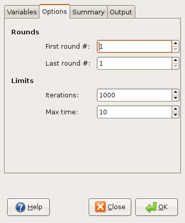
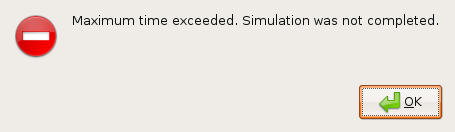
The second pair of options are the number of iterations and the Max time. In a simulation, each iteration is the equivalent of a sample. A sample from a random distribution is taken for each of the input values (as specified in the Variables tab) and the resulting output value(s). The more iterations, the better the estimate of the output value. However, this also takes more time to run. A Max time value is specified in seconds where the simulation will end without output if an individual simulation takes longer than the Max time allotted. If this occurs (see Figure 6-7), the options are to either increase the Max time value, or decrease the number of iterations. A more drastic option is to change the model so that fewer calculations or samples of random numbers need to be made.
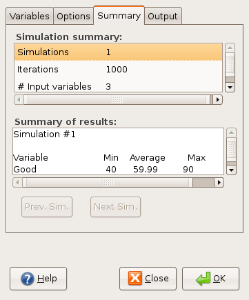
The next tab is the Summary. There are two boxes in this tab, the Simulation Summary and the Summary of results (see Figure 6-8). In simulation summary, there is a description of the simulation parameters.
Due to the random nature of the simulation, the output may vary between simulation runs).
- Simulations: Number of rounds as determined in the Simulation Options box.
- Iterations: Number of iterations in a single simulation round.
- # input variables: Number of random numbers sampled for each iteration.
- # output variables: Number of outputs recorded for simulation
- Runtime: Runtime of simulations in seconds.
- Run on: Date and time simulation was run.
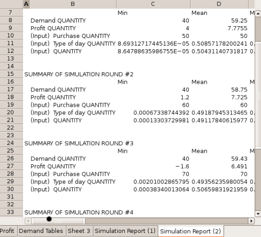
In the summary of results window, there are summary statistics for each round of the simulation. If multiple rounds were done, the results of each round can be browsed by using the 'Prev. Sim.' and 'Next Sim.' buttons below the Summary of results box. For each output and input variable, the summary shows the Min, Average and the Max value across the iterations for that round of the simulation. Note that for the input variables, this shows the random number that is the average, max and min. If the statistics on intermediate values, such as a cost distribution, was desired, these intermediate values should be added to the list of output variables.
The last tab is labeled 'Output'. This tab identifies the location where the output table will be generated. There are two sets of options, first the Output Placement then Output Formatting as shown in Figure 6-9.
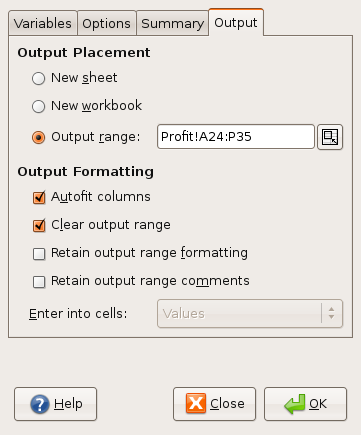
The default output placement is 'New sheet'. This will create a new sheet in the Gnumeric workbook labeled 'Simulation Report (1)', where '1' can be replaced with another number if a tab labeled 'Simulation Report (1)' already exists. The option 'New workbook' creates a Gnumeric workbook named 'Book2.gnumeric' with a tab labeled 'Simulation Report.'
The third option is to embed the output table into an existing worksheet. This is done by specifying the 'Output range'. Note that the output range must be large enough to include the entire table, including heading information. For a single round this requires 11 rows and 16 columns. For example, the range Profit!A24:P35 would contain the statistics for one round with the three input variables and two output variables. As input and output variables change, or the number of rounds of the simulation change, the number of rows required will change.
For output formatting, their are four options.
- 'Autofit columns' automatically makes each column long enough to include the largest entry in that column. Note that column 'A' in the resulting spreadsheet used to save run information such as date and time and is kept narrow.
- 'Clear output range' is in effect if the Output Placement option chosen is Output range. It clears the selected cells in the spreadsheet before putting the output table in its place.
- 'Retain output range formatting' retains formatting for cells such as number formatting.
- 'Retain output range comments' retains comments that have been placed in output cells. This is most useful when the input and output variables remained the same.
6.4.4. Simulation output
The simulation output provides statistics on the output and input variables for each round. The statistics are calculated over the iterations in a single round of the simulation. These statistics for each variable are:
- Variable type and name - input variables are labeled as '(Input)'.
- Min – Minimum value of variable among iterations of round.
- Mean – Arithmetic mean of variable among iterations of round.
- Max – Maximum value of variable among all iterations of round.
- Median – Median of variable among iterations of round.
- Mode – Mode value among iterations of round. For the input variable, this will be “#N/A”.
- Std. Dev. - Standard deviation of the variable.
- Variance – Second moment of variable.
- Skewness - Third moment of variable.
- Kurtosis – Fourth moment of variable.
- Range – Difference between min and max of variable among iterations of the round.
- Count – Number of iterations in round.
- Confidence (95%) - 95% confidence interval of value, centered on mean.
- Lower Limit (95%) - Lower limit of 95% confidence interval of the value, centered on the mean.
- Upper Limit (95%) - Upper limit of 95% confidence interval of the value, centered on the mean.

The output will include a heading, then a table for each round of the simulation. Judicious choice of output variables will also include any intermediate values of interest in the simulation in this table. Each row of the output table has statistics of the values of a variable over the iterations of the simulation as shown in Figure 6-10.
The output will be of the input variables and the output variables that were variables tab of the Simulation window . For the input variables, the output will be the statistics of the random variable used in modeling the input variables. For the output variables, the statistics will be of the output variable. These statistics, in particular the standard deviation and confidence interval, should be examined to ensure the simulation was at a precision adequate for the purpose. Some notes on how to use these statistics for refining the simulation design can be found in Section 6.4.6 ― Determining the number of iterations.
6.4.5. Using SIMTABLE
The SIMTABLE function is intended to change a variable in the simulation so that each round of the simulation can be used to evaluate a different scenario. This automates the use of simulation for what-if questions or to create a set of possible outcomes to a situation.
In this example, we will use the SIMTABLE function to find the optimal quantity of newspapers to buy. For the purchase quantity in our spreadsheet, we will replace '50' with the following formula in Profit!B16:
Profit!B16 = SIMTABLE(50,60,70,80,90)
Each entry in the list of the SIMTABLE arguments is a value that will be used for the purchased quantity. Each entry corresponds to one round of simulation, as used in Figure 6-6. In this example there are 5 entries to the SIMTABLE list, so '5' will be entered into the 'Last Round #' option in the Options tab of the Simulation dialog.
When this simulation is run with 5 rounds, the summary of results will have one entry for each round, with each round using a different entry from the SIMTABLE function for the purchase quantity. The results for the various rounds can be previewed using the 'Prev. Sim.' and 'Next Sim.' buttons. The output also has one table for each round of the simulation.
As seen in Figure 6-11, each value in the original SIMTABLE statement corresponds to a simulation round, with the Purchase Quantity taking on the value from the SIMTABLE list. The analyst can then record the Profit statistics (mean, variance, skewness, kurtosis, 95% confidence intervals) and determine if the simulation results are of sufficient resolution for the analysts purposes.
The use of SIMTABLE to change parameters within the simulation provides a convenient method to do what-if analysis, and analyze the results as a whole.
6.4.6. Determining the number of iterations
In simulation, one major question is how many iterations are needed to reach a chosen level of precision in the results. Simulation as a tool provides an approximation of the actual relationship between the input and output variables. The precision of the approximation is based on the number of iterations of the simulation done. More iterations in the sample lead to greater precision. But the relationship between iterations and precision depends on the relationship between the variables in the precision. In addition, the analyst must decide which output variable is the variable of interest, and what degree of precision is required. The next step is to determine a sufficiently large number of iterations R be used to satisfy:
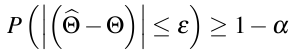
Where Θ-hat is the estimate of the mean, Θ is the actual mean, ε is the specified error, and (1-α) is the probability that the estimate is within ε of the actual value (i.e. the (1-α) confidence interval). Common values of (1-α) are 95% and 99%. The Simulation Report from Gnumeric includes values for the 95% confidence interval as shown in Figure 6-10.
The general procedure is as follows:5
- Run simulation for a sample of R0 iterations. The default value in Gnumeric is 1000, set in the options tab of the Simulation menu, Figure 6-6.
- Take the sample variance S02 from the simulation output spreadsheet and determine the sample standard deviation S0 (see Figure 6-10).
- Using
zα/2
as the z-value of the
(1-(α/2))
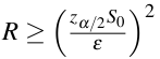
percentile of the standard normal distribution, set the initial estimate of the number of iterations required as the smallest integer
R
such that
. Note that if R0 is small, it would be more appropriate to use the student's t-distribution of tα/2, R0 instead of zα/2 .Iterations required for simulation
In this example, to estimate the profit to within ε=0.05 , first run the simulation with 1000 iterations and a purchase quantity of 50 results in the following
| Mean | Variance | Confidence (95%) | |
| Demand QUANTITY | 59.19 | 152.4 | 0.64 |
| Profit QUANTITY | 7.85 | 2.51 | 0.08 |
Taking the variance of the table, and setting ε=0.05 and α=0.05 , lookup zα/2 from a standard normal table. zα/2=1.96 so we have
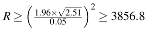
Therefore, the minimum number of iterations is 3857. The simulation can then be re-run with 3857 iterations to create a 95% c.i for profit where ε <=0.05 In this example with 3857 iterations, we get the following Simulation Report table:
| Mean | Variance | Confidence (95%) | |
| Demand QUANTITY | 59.11 | 163.9 | 0.34 |
| Profit QUANTITY | 7.72 | 2.88 | 0.04 |
As expected, the 95% Confidence interval for Profit is less than 0.05. For the newsvendor example, the next step would be to look at the confidence intervals of the profit for all values of purchase quantity, and verify that this confidence interval is adequate for the decision to be made.